Atam Oguz Erkara

Classroom Topic

Support Vector Machines

This page gives a simple explanation of Support Vector Machines. The topic was originally prepared for an Imaging Physics course presentation. The goal was to explain what SVM is, what it is useful for, and how it can classify data through an intuitive penguin dataset example.

Basic Idea

SVM is a classification method. Imagine two groups of data points. Many lines may separate them, but SVM searches for the line that separates them with the widest possible gap. That gap is called the margin. The closest points around this margin are called support vectors.

A simple way to imagine it is a road between two groups. SVM tries to make that road as wide as possible while still keeping the two groups on different sides. Logistic regression focuses on probability. SVM focuses on the boundary and the margin.

Penguin dataset illustration

Explanation of SVM Concept

1. SVM as a supervised classification method+

Support Vector Machine is a supervised classification method. It learns from labelled examples and tries to separate data points into correct classes. The main idea is not to predict probabilities directly, but to find a strong decision boundary between classes.

Here, x represents the input features and y represents the class label. For a simple two class problem, labels can be written as negative and positive classes.

SVM supervised classification idea
2. Many lines can split the data+

If the data has two features, we can draw it on a two dimensional graph. Several lines may separate the classes. However, SVM does not only ask whether a line separates the data. It asks which separating line is the best one.

This is the intuitive starting point. Many answers can work, but SVM searches for the most reliable separating boundary.

Different possible decision boundaries
3. Margin, hyperplane, and support vectors+

The best boundary is the one with the widest margin. The margin is the distance around the separating boundary. The closest points to this boundary are called support vectors, and the main separating boundary is called the hyperplane.

Mathematical form

Decision boundary:
wᵀx + b = 0

Margin boundaries:
wᵀx + b = +1
wᵀx + b = −1

Margin width = 2 / ||w||

This is the mathematical version of the widest road idea. SVM tries to keep the closest points from both groups as far as possible from the separating boundary.

SVM margin hyperplane and support vectors
4. Penguin dataset demonstration+

The practical example used a penguin dataset with Adelie, Gentoo, and Chinstrap penguins. To make the first demonstration simple, Chinstrap was removed and the model focused on separating Adelie and Gentoo penguins.

The dataset contains physical measurements such as bill length, bill depth, body mass, island, and sex. This makes it useful for a visual classification example.

Penguin dataset description
5. Feature selection with bill length and bill depth+

Bill length and bill depth were selected because they are easy to visualize in two dimensions. In this feature space, each penguin becomes one point on the graph.

The classifier does not understand penguins directly. It only sees numerical features. Good feature selection makes the separation clearer.

Bill length and bill depth distribution
6. Linear SVM training+

A linear Support Vector Classifier was trained on the selected features. Linear means the classifier searches for a straight separating boundary between the two penguin groups.

Linear SVM is the simplest case and fits the visual explanation well because the boundary can be drawn as a line.

Linear SVM visualization
7. Prediction example+

After training, the model can classify a new penguin measurement. A point close to the decision boundary is useful because it tests whether the learned separation is meaningful.

Mathematical form

Decision rule:
f(u) = wᵀu + b

if f(u) ≥ 0  →  class +1
if f(u) < 0   →  class −1

A new point u is compared with the learned direction w. The sign of the result decides the predicted class.

SVM prediction point
8. C parameter and misclassification+

The C parameter controls how strict the classifier should be. A lower C allows more tolerance. A higher C punishes misclassification more strongly.

Mathematical form

Soft margin objective:
minimize  1/2 ||w||² + C Σᵢ ξᵢ

small C  →  softer margin
large C  →  stricter margin

This parameter is important because real data is rarely perfect. Sometimes allowing a few mistakes gives a better general boundary.

C parameter in SVM
9. Soft margin condition+

Soft margin SVM allows some samples to violate the margin. This is useful when the dataset contains noise, outliers, or overlapping classes.

Mathematical form

yᵢ(wᵀxᵢ + b) ≥ 1 − ξᵢ
ξᵢ ≥ 0

The slack variable ξᵢ measures how much a sample violates the margin. This makes SVM more realistic for imperfect real world data.

Soft margin SVM
10. Hard margin condition+

Hard margin SVM does not allow margin violations or misclassifications. It assumes that the data can be perfectly separated by a decision boundary.

Mathematical form

yᵢ(wᵀxᵢ + b) ≥ 1

There is no slack variable in hard margin SVM. Every training sample must stay on the correct side of the margin.

Hard margin SVM
11. Higher dimensional classification+

SVM is not limited to two features. More features can be added, such as body mass. With three features, the separating boundary becomes a plane. With four or more features, visualization becomes difficult but the same idea still works.

The visual object changes from a line to a plane and then to a hyperplane, but the goal remains the same: separate the classes with a strong margin.

SVM higher dimensional plane
12. Multi class classification+

SVM is naturally easier to explain as a two class method. However, it can also classify more than two classes by comparing classes through smaller binary classification problems.

For the penguin dataset, this can mean Adelie versus the rest, Gentoo versus the rest, and Chinstrap versus the rest.

SVM multi class classification
13. Kernel trick+

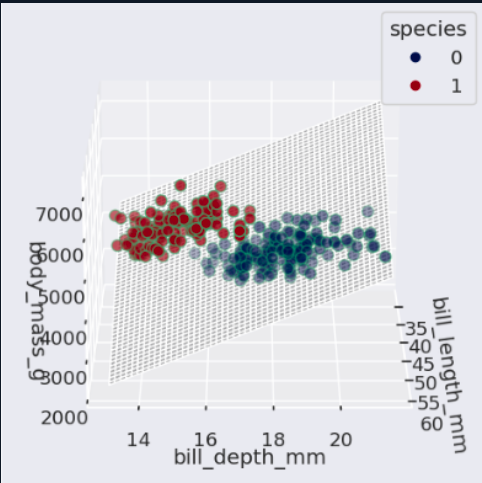
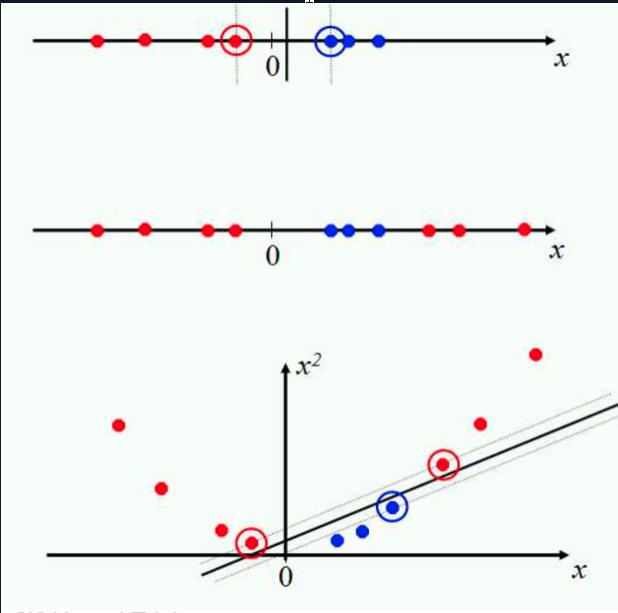
If the data cannot be separated with a straight line, SVM can use a kernel. The kernel trick changes the perspective of the feature space so that a separation becomes possible in another representation.

Mathematical form

Dual form:
L = Σᵢ αᵢ − 1/2 ΣᵢΣⱼ αᵢαⱼyᵢyⱼ(xᵢᵀxⱼ)

Kernel replacement:
xᵢᵀxⱼ  →  K(xᵢ, xⱼ)

Decision with kernel:
f(u) = Σᵢ αᵢyᵢK(xᵢ, u) + b

Common kernels:
Linear:      K(x, z) = xᵀz
Polynomial:  K(x, z) = (xᵀz + c)ᵈ
RBF:         K(x, z) = exp(−γ||x − z||²)

The kernel trick works because the dual formulation depends on dot products. Replacing the dot product with a kernel function allows SVM to handle non linear separation.

SVM kernel trick
14. Application example in remote sensing+

The presentation also discussed remote sensing image classification. In that study, SVM was compared with other methods for classifying land information from image based features.

This shows that SVM is not limited to classroom examples. It can also be applied to image related classification tasks and remote sensing applications.

15. Short history+

The story of Support Vector Machines is strongly connected to Vladimir Vapnik and statistical learning theory. The basic idea did not appear suddenly as a finished modern tool. It developed over many years. First came the theoretical foundation. Later, stronger computers and real benchmark problems made the method practically testable. In the early 1990s, kernel based SVMs became especially important because they allowed non linear classification. This helped SVM become visible in problems such as handwriting recognition, image classification, and other pattern recognition tasks.

This is why SVM feels both mathematical and practical. It is a theoretical idea that became powerful when the computational environment finally caught up with it.

Strengths

  • Good option for small and medium sized datasets.
  • Works well with high dimensional feature spaces.
  • Strong margin based classification logic.
  • Kernel functions make it flexible for non linear data.

Limitations

  • Can become computationally expensive on large datasets.
  • Kernel choice affects the result strongly.
  • Hyperparameter tuning may require extra testing.
  • Results are harder to visualize in four or more dimensions.

References and Materials

These sources were used while preparing the SVM explanation, especially for the kernel trick, kernel types, remote sensing example, video material, and penguin dataset.

© 2026 Atam Oguz Erkara